Surface Flux Transport (SFT) describes the latter part of the dynamo
process, in which the flows on the surface of the Sun transport the magnetic flux from the
active region belts to the poles. During solar maximum the
previous cycle's polar fields are cancelled and a new poloidal
field with the opposite polarity begins to grow. At solar minimum, the strength of this new
poloidal field becomes the seed to the next solar cycle.
SFT begins with the emergence of bipolar magnetic active regions with the characteristic Hale’s
polarity and Joy’s Law tilt (Hale et al. 1919; Howard 1991). Initially, the active regions emerge
at about 30° latitude. As the cycle progresses, they emerge at progressively lower latitudes,
eventually stopping near the equator. The magnetic flux in the active regions is shredded off
by turbulent convective motions (over a period of a few days or weeks) and is dispersed into the
surrounding plasma. The dispersed flux is then transported by the surface
flows: differential rotation, meridional circulation, and the turbulent cellular motions of
convection. The weak magnetic elements are carried to the edges of the convective structures
(granules and supergranules) by flows within those convective cells, forming a magnetic network.
Once concentrated in the magnetic network, the flux is then carried (along with the convective
cells) by the axisymmetric differential rotation and meridional circulation.
While the majority of the active region flux will cancel with the opposite polarity from the
active region itself or with future active regions, some residual flux remnants will remain.
The lower latitude leading polarity flux remnants will eventually cancel across the equator,
while the higher latitude following polarity flux remnants migrate to the poles. The following
polarity flux cancels with the original global poloidal field and creates a new poloidal field
with opposite polarity, from which the new solar cycle is born.
Most previous SFT models have been highly parameterized, in particular with respect to active
region emergence, the meridional flow, and the convective motions. Previous models have been
restricted to simulating active region emergence by inserting artificial bipolar active region
sources (though some have been based on observed active regions). The adopted meridional flow
profiles (sharply peaked at low latitudes, stopping short of the poles, exaggerated variations
around active regions) deviate substantially from the observed profiles. Additionally, these
models have typically neglected the variability in the meridional flow altogether (the
meridional flow is faster at solar cycle minimum and slower at maximum). Furthermore, virtually
all previous models have parameterized the turbulent convection by a diffusivity with widely
varying values from model to model.
When we set out to create our SFT model, the Advective Flux Transport (AFT) model, our primary
goal was to create the most realistic SFT model possible by incorporating the observed active
regions and surface flows directly, with minimal parameterizations. The AFT model uses the
measured axisymmetric flows along with a convective simulation to explicitly model the surface
flows produced by the convective flows. The convective simulation uses vector spherical harmonics
to create a convective velocity field that reproduces the spectral characteristics of the
convective flows observed on the Sun. The spectral coefficients evolve, giving the simulated
convective cells finite lifetimes and moving them with the observed differential rotation and
meridional flow. Strong magnetic fields on the Sun inhibit convection; therefore when the flow
velocities are employed, they are dampened where the magnetic field is strong. This magnetic
field strength dependent effect is difficult to reproduce with the diffusivity used in other
models. Advecting the flows with the simulated convection allows the model to surpass the
realism that can be obtained by using a diffusivity coefficient.
Magnetic sources can be incorporated in two different ways: either by manually inserting
bipolar active regions (e.g., using active region databases like NOAA to insert flux daily as the
active region grows) or by assimilating magnetic data directly from magnetograms. This gives the AFT
model additional flexibility. While manual insertion allows the AFT model to be used to investigate
flows and to make predictions, the assimilation process provides the closest contact to the
observations, producing the most accurate synchronic maps of the entire Sun. These maps, referred
to as the Baseline data set, can be used as a metric for evaluating SFT or as source data for
models that extend into the solar atmosphere and the heliosphere.
Discover AFT: Polar Field Predictions!
We have demonstrated the power of the AFT model by simulating Cycle 23 during the polar field reversal
(
details in this paper). Starting with data 3 years ahead of the reversal, we were able to predict
the timing of the field reversal to within four months, with four out of five predictions accurate to
within a month. Furthermore, we found that our predictions for the polar field evolution stayed in
remarkably good agreement with the baseline through to the end of the prediction, an additional 3 years
after the reversal, demonstrating the ability to accurately predict the evolution of the Sun’s dipolar
magnetic field several years in advance. The increase in the spread of the measurements over time highlights
the stochastic nature and important role that supergranules play in the transport of flux.
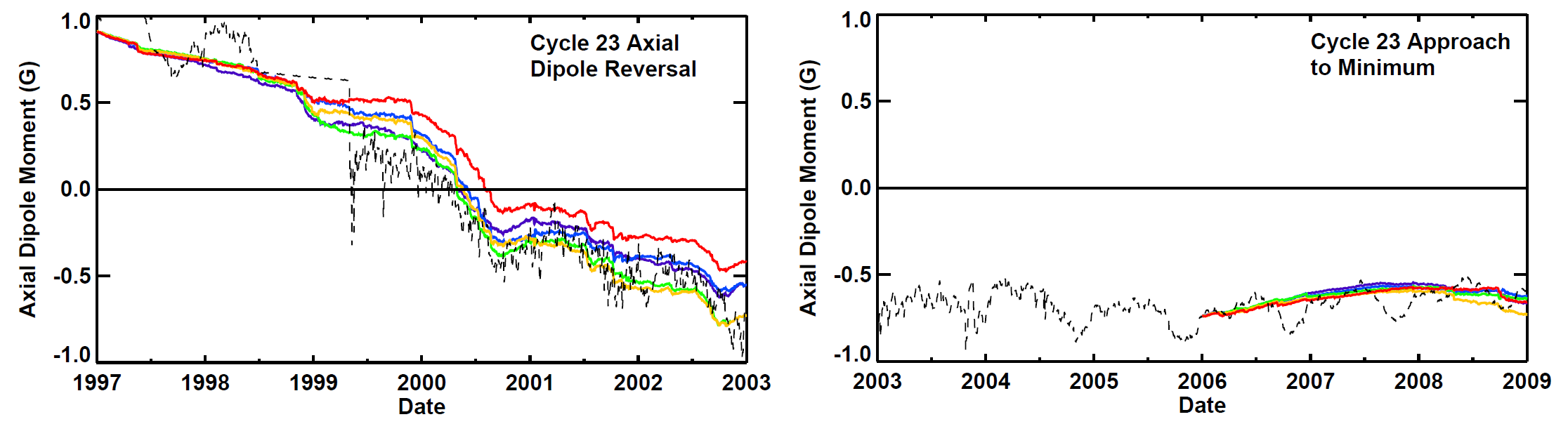
Solar Cycle 23 Simulations. Solar Cycle 23 simulations (each color represents a different realization
of the convective pattern) of the axial dipole moment evolution are compared to MDI observations (black).
(Note: the annual signal in the MDI data is due to instrumental effects.) These predictions were made
using Cycle 17 active region data as magnetic sources. The Solar Cycle 23 polar field reversal is shown
on the left. The approach to the Solar Cycle 23/24 minimum is shown on the right.
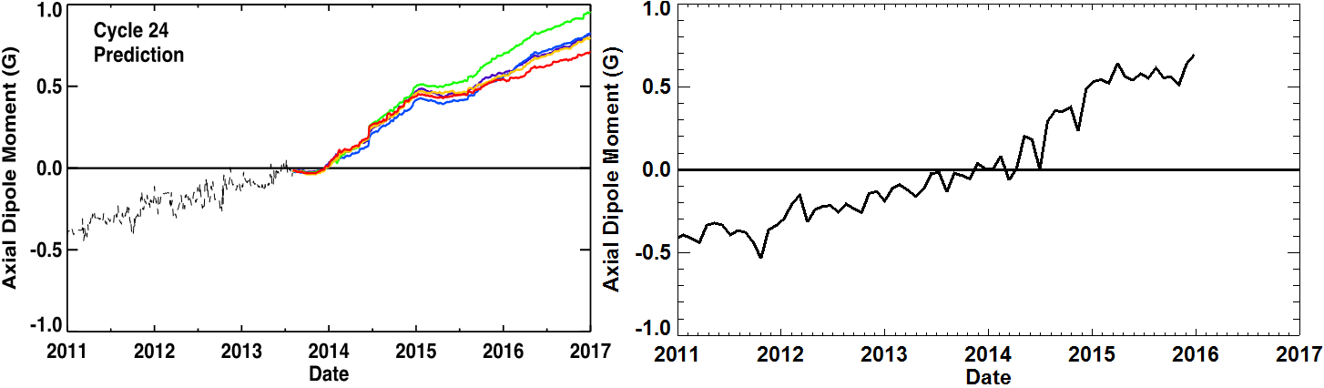
We went on to use the AFT model to predict the Solar Cycle 24 axial dipole moment reversal and subsequent
magnetic field buildup, using Solar cycle 14 active regions as proxies for the continued active region
emergence. Comparison of this prediction with the evolution of the axial dipole that has since occured,
show remarkable agreement. Both feature a relapse in the reversal, leading up to the end of 2014, followed
by a steady rise until the beginning of 2015. The axial dipole then plateaus defore taking off again at the
beginning of 2016.
Solar Cycle 24 Prediction. The axial dipole moment for the solar cycle 24 polar field reversal as predicted
(left) and as observed with HMI magnetograms (right). The different colored tracks in the
prediction represent different realizations of the convective motions.
Our prediction for Solar Cycle 25 can be found here.
Discover AFT: Active Region Simulations!
In addition to polar field evolutions, we have also investigated the finer details of individual active region
evolution in the AFT model(
details in this paper). We compared the total unsigned magnetic flux estimated from EUV 304 Å flux-luminosity
relation directly to the total unsigned magnetic flux from the AFT baseline model. We found that the AFT model
can accurately reproduce the active region evolution when the active region is not being observed by HMI and
the model is operating without assimilation. Additional flux may emerge, however, while the active region is
on the far-side. The AFT assimilation process corrects for this new emergence when this flux is observed by HMI
and rotates over the East limb.
AFT Active Region Evolution. The left plot shows the flux obtained from the 304 proxy and the flux
for two area integrations of the AFT model (red and orange) for Active Region 11158 . Grey areas mark the times
when the active region is on the Earth side, when data from HMI magnetograms is being assimilated. The EUV and AFT
maps at the time near peak 304 °A intensity is shown on the right.
 Solar Cycle Science
Discover the Sun!
Solar Cycle Science
Discover the Sun!